Normally, the computation of incremental rotation would entail
a complete recasting of the ![]() rays. However, the ADRT technique
defines a way to store some of the intermediate data produced in
ray casting at a given orientation for use in computing incremental
rotations. Observe, for example, the segments at neighboring orientations
shown in Figure 5. Large sets of voxel samples are shared between
the neighboring rays.
Thus, if a ray is divided into shorter segments and the rendering of these
segments are stored, they might be used to construct rays at many
different rotations. This idea has been used to compute projections
in 2D images [22] (i.e., for the ADRT),
and extended to 3D ray tracing for volume visualization in [23,24].
rays. However, the ADRT technique
defines a way to store some of the intermediate data produced in
ray casting at a given orientation for use in computing incremental
rotations. Observe, for example, the segments at neighboring orientations
shown in Figure 5. Large sets of voxel samples are shared between
the neighboring rays.
Thus, if a ray is divided into shorter segments and the rendering of these
segments are stored, they might be used to construct rays at many
different rotations. This idea has been used to compute projections
in 2D images [22] (i.e., for the ADRT),
and extended to 3D ray tracing for volume visualization in [23,24].
![]()
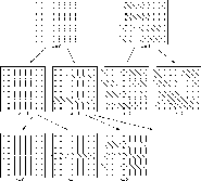
Figure 5. Illustration of how segment-sharing in ADRT helps
compute rotation views efficiently (2D case, n=8). The figure depicts
a slice through the image data. A ray cast for view angle ![]() shares much data (4 of 8 voxels) with a ray cast for the rotated
view angle
shares much data (4 of 8 voxels) with a ray cast for the rotated
view angle ![]() .
.
First, for simplicity, consider the tracing of n rays thro- ugh a 2D
image of size ![]() , where n is a power of two.
The ADRT
algorithm constructs rays at n different angles simultaneously, in
the range [0,
, where n is a power of two.
The ADRT
algorithm constructs rays at n different angles simultaneously, in
the range [0, ![]() ]. All rays begin on a pixel in the bottom row,
and end on a pixel in the top row. Rays are computed hierarchically.
First, a set of 2-pixel line segments are constructed. These
2-pixel segments are then used to construct 4-pixel segments,
and so forth, concluding with the combination of
]. All rays begin on a pixel in the bottom row,
and end on a pixel in the top row. Rays are computed hierarchically.
First, a set of 2-pixel line segments are constructed. These
2-pixel segments are then used to construct 4-pixel segments,
and so forth, concluding with the combination of ![]() -pixel segments
to form the n-pixel rays. Define the x-displacement of a
segment, a,
as the difference in x-coordinates of the segment's lower and upper
end points. In the first pass, 2-pixel segments with x-displacements
of 0 and 1 are constructed, starting in every other row, as shown in
Figure 6. In the second pass, 4-pixel segments
with a = 0, 1, 2, and 3 are constructed from the 2-pixel segments,
in every
-pixel segments
to form the n-pixel rays. Define the x-displacement of a
segment, a,
as the difference in x-coordinates of the segment's lower and upper
end points. In the first pass, 2-pixel segments with x-displacements
of 0 and 1 are constructed, starting in every other row, as shown in
Figure 6. In the second pass, 4-pixel segments
with a = 0, 1, 2, and 3 are constructed from the 2-pixel segments,
in every ![]() row (see Figure 6). In particular, the 2-pixel segments
with x-displacement 0 (x-displacement 1) are used to compute the
4-pixel segments with a = 0 and 1 (a = 2 and 3). Let
row (see Figure 6). In particular, the 2-pixel segments
with x-displacement 0 (x-displacement 1) are used to compute the
4-pixel segments with a = 0 and 1 (a = 2 and 3). Let ![]() represent the
represent the ![]() -pixel segment computed in pass i, with lower end
point
-pixel segment computed in pass i, with lower end
point ![]() and an x-displacement of a. Then
and an x-displacement of a. Then
![]() ,
where * denotes a rendering operation.
,
where * denotes a rendering operation.
The ADRT algorithm for angles in the range ![]() is shown below (Algorithm 1).
is shown below (Algorithm 1).
Algorithm 1. ADRT computation for ![]() .
.
Initialize ![]() :
:
![]() for
for ![]()
![]() for
for ![]() ,
, ![]()
Compute the RT:
for i = 1 to ![]()
for a = 0 to ![]()
for y = 0 to ![]() step
step ![]()
for x = 0 to 2n-1
![]()
The pixel values ![]() are stored in
are stored in
![]() , and the image is padded with an additional
, and the image is padded with an additional ![]() zeroes on the right side and computed cyclically (modulo 2n) so
that lines that ``fall off" the sides continue by adding zeroes to
their sum. (This avoids the need to check for image boundaries,
simplifying the algorithmic description.) After
zeroes on the right side and computed cyclically (modulo 2n) so
that lines that ``fall off" the sides continue by adding zeroes to
their sum. (This avoids the need to check for image boundaries,
simplifying the algorithmic description.) After ![]() passes, the projection data resides in
passes, the projection data resides in ![]() , where
the projection angle is
, where
the projection angle is ![]() and the ray
passes through
and the ray
passes through ![]() .
.

Figure 6. Hierarchical construction of rays in ADRT
(2D case). At stage i, ray segments of length ![]() are constructed.
are constructed.
By applying Algorithm 1 a slice at a time to the viewing
parallelepiped, a restricted set of parallel projections about
one of the axes can be computed at once, at up to n
different angles.
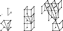
The extension to general orientations (both rotation and tilt not equal to
0) is straightforward, as shown in Figure 7. Up to ![]() different orientations can be computed simultaneously, as shown
below in Algorithm 2.
In each pass, the amount of work doubles,
as does the amount of data produced. Thus, the run time is dominated
by the last pass and requires
different orientations can be computed simultaneously, as shown
below in Algorithm 2.
In each pass, the amount of work doubles,
as does the amount of data produced. Thus, the run time is dominated
by the last pass and requires ![]() operations. This means that each
view is computed
in an average of
operations. This means that each
view is computed
in an average of ![]() operations, a factor of n faster than computing
them
independently. However, direct implementation of Algorithm 2 carries a large
start-up penalty. In the next subsection, we describe a data structure that
uses the approximate sampling technique of Algorithm 2, without incurring
such a large cost to initialize the structure.
operations, a factor of n faster than computing
them
independently. However, direct implementation of Algorithm 2 carries a large
start-up penalty. In the next subsection, we describe a data structure that
uses the approximate sampling technique of Algorithm 2, without incurring
such a large cost to initialize the structure.
Algorithm 2. Approx. Volume Rendering Computation.
Initialize ![]() :
:
for z = 0 to n-1
for x = 0 to 2n-1, for y = 0 to 2n-1
![]()
for x = 0 to ![]() , for y = 0 to n-1
, for y = 0 to n-1
![]()
Compute ![]() projections:
projections:
for i = 1 to ![]()
for a=0 to ![]() , for b=0 to
, for b=0 to ![]()
for x=0 to 2n-1, for y=0 to 2n-1
for z=0 to ![]() step
step ![]()
![]()
![]()
![]()
In this approximate sampling technique, the maximum distance of any sample
point from the intended ray
can be shown to be upper bounded by
![]() [23]. Further, this
bound is not tight: while the error is observed to grow as
a function of
[23]. Further, this
bound is not tight: while the error is observed to grow as
a function of ![]() , the constant appears to be smaller than
0.35. In particular, for n=64 the maximum distance of any sample point
from its intended line is
, the constant appears to be smaller than
0.35. In particular, for n=64 the maximum distance of any sample point
from its intended line is ![]() units, and for n=32 it is
units, and for n=32 it is ![]() . By
comparison, for standard nearest-neighbor voxel sampling, the sample points are within
. By
comparison, for standard nearest-neighbor voxel sampling, the sample points are within
![]() units.
units.

Figure 7. Generalization of ADRT ray construction for 3D. (Partial figure only for clarity).